Harmonics and Timbre

What makes the sound of a violin different from that of a piano, even when playing the same note? The answer lies in timbre, the quality that distinguishes instruments. In this post, we’ll explore how timbre arises from the combination of fundamental frequency and harmonics, and how this characteristic defines the unique sound of each instrument.

Let’s make a few considerations. In the previous post, we identified a function, $y(t)$, which uniquely determines the shape of a sound wave, and therefore – as we will now say, though we will explore this further – the same note.

This function is defined by amplitude, frequency, and phase; the latter, however, is a rather abstract concept that, while it impacts the sound wave, doesn’t change its essential nature. Now, one might ask what difference there is between an A played on a trumpet, a bass, a piano, or a synth. After all, if I have a function that uniquely identifies the waveform, it should always produce the same note, given the same frequency and amplitude.

Evidently, something is missing in the model. In fact, in the previous article, we mentioned, besides amplitude and frequency, a third component: timbre. Timbre is what allows us to distinguish between different instruments playing the same note at the same pitch and intensity, so it’s the characteristic missing in the initial model.

“Musicians” (in reality, anyone) define an octave as the musical interval between two notes that sound similar, but one is higher or lower than the other. If you play an A on a piano and then the next A, those two notes are an octave apart. Even though they sound at different pitches, we perceive them as “the same note” on two different levels.

For the purpose of this post, an octave is the interval between two notes where the frequency of the second note is exactly double that of the first. This 2:1 ratio is what makes the two notes perceived as “the same note,” but at different pitches. For example, if a note has a frequency of 440 Hz (the standard A), the note an octave higher will have a frequency of 880 Hz. This harmonic relationship between frequencies is what defines the octave.

Digression

Despite the vast differences between musical systems around the world, the octave serves as a common reference point across all cultures. Each musical tradition has developed its own scales and tuning systems. For example, in modern Western music, we use a seven-note diatonic scale, while in other cultures, pentatonic scales (with five notes) or systems that include microtones—intervals smaller than our semitones—are used. However, regardless of the number of notes in a scale or how they are tuned, the octave remains a fundamental element.

In all musical traditions, two notes separated by an octave are perceived as “the same” note, just at a different pitch. For example, in a Chinese pentatonic scale, when a base note is played followed by a note one octave higher, the second note is recognised as the same, just higher in pitch. Similarly, in Indian music, which can have up to 22 divisions within the octave (called “shruti”), a note and its octave maintain a relationship of similarity in how they are perceived.

This universal recognition of the octave is due to the way our auditory system responds to sound frequencies. No matter how different African, Japanese, Arabic, or European music may seem, the octave is a constant that transcends cultural differences.

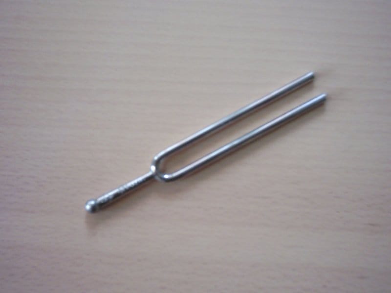
The function $y(t)$ doesn’t fully define a note as we would expect it in real life, but rather the note in its purest (or almost pure) form. Think of it as the sound produced by a tuning fork, for example—although even this isn’t a “pure” note in the sense of it being just the fundamental frequency of a note.

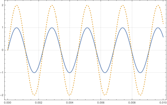
Figure 1: the same note (A, in this case) played at two different volumes.

The code generating the above is:

F[t_, freq_, phase_, amp_] := amp*Sin[2*Pi*freq*t + phase]
freq = 440;
phase = 0;
ampl = 1;
tmax  = 0.01;
Plot[{F[t, freq, phase, ampl], F[t, freq, phase, 2*ampl]}, {t, 0, 
  tmax}, PlotRange -> All, AxesLabel -> {"Time (s)", "Amplitude"}, 
 PlotLegends -> {"F(t, freq, phase, ampl)", 
   "F(t, freq, phase, 2ampl)"}, PlotStyle -> {Thick, Dashed}, 
 PlotTheme -> "Detailed", PlotPoints -> 100, MaxRecursion -> 2, 
 ImageSize -> Large]

This justifies calling $y(t)$ the fundamental frequency of the note, which is only an idealised model. The instruments we’re used to produce other sounds when we play a note.

Movie 1: a pure A waveform

The code that generated this was

duration = 2
sound = Play[Evaluate[F[t, freq, phase, ampl]], {t, 0, duration}];
Export["./wave_sound.wav", sound]
animation = 
  Table[Plot[F[t, freq, phase, ampl], {t, 0, 0.01}, 
    PlotRange -> {{0, 0.01}, {-1, 1}}, 
    PlotLabel -> "Waveform of A 440Hz", 
    AxesLabel -> {"Time (s)", "Amplitude"}, 
    Epilog -> {Red, PointSize[Large], 
      Point[{tCurrent, F[tCurrent, freq, phase, amp]}]}], {tCurrent, 
    0, 0.01, 0.0001}];
Export["./wave_animation.gif", animation]

and then combining it all together with:

ffmpeg -i wave_animation.gif -i wave_sound.wav -c:v libx264 -c:a aac -strict experimental output_movie.mp4

Similarly, we created a more complex wave, summing several harmonics

Movie 2: a more complex soundwave rooted on the A key

As we mentioned, every real-life sound contains both the fundamental harmonic and other sounds, hence additional waveforms. Similarly, these sounds will have their own fundamental harmonic and a series of other waveforms. We can measure that the fundamental frequency of these notes is itself an integer multiple of the frequency of the originally played note.

In reality, the other waveforms present are not always perfect multiples of the fundamental frequency but follow a hierarchy related to the physics of the instrument that produces the sound. We will explore this in more detail later, but for now, let’s consider it a minor point.

In general, the ear doesn’t perceive harmonics as separate notes, but they influence the way the note “sounds.” They are responsible for the richness, brightness, or fullness of the sound. For example, a violin might sound brighter because it has stronger higher harmonics, while a flute sounds purer and “softer” because it has fewer harmonics compared to instruments like a guitar or a piano. A synth can modulate harmonics to create very different sounds, ranging from soft tones to metallic or sharp ones.

Thus, harmonics give character and depth to the sound. Without harmonics, the note would sound very “flat” or artificial, like a pure sine wave.

We have identified the fundamental frequency (where ff is the frequency of the note, for example, 440 Hz for A). $A0​$ is the amplitude of the fundamental frequency, and $phi_0$​ is the initial phase:

$$y(t)=A_0\sin(2\pi f t+\phi_0)$$

and the harmonics, that being waveforms can be modelled as

$$ \psi_k(t) = \alpha_k \sin(2\pi kft +\phi_k ), \quad k=1,2,\dots $$

being $\alpha_k$ the amplitude of the $k$-th harmonic and $\phi_k$ its phase.

The series of harmonics is theoretically infinite, with each successive harmonic having a frequency that is an integer multiple of the fundamental frequency ($kf$). Therefore, a note produced by an instrument can be modeled as:

$$ Y(t)=y(t)+ \sum_{k>1} \psi_k(t) $$

The fundamental frequency plus the various harmonics define the timbre of the sound, which is what distinguishes different instruments. Not all instruments create the same harmonics with the same frequencies or decay rates, which explains the differences between instruments. In other words, the various $\psi_k$​ are uniquely determined not only by the type of instrument but by the specific instrument itself. For instance, a Stradivarius violin or Brian May’s guitar have sounds distinct from all other instruments of the same model and often even from those of the same brand!

In the next post, we will discuss the auditory system of both animals and humans.