Exploring Musical Frequencies: The 12-Tone Equal Temperament and Modern Tuning Systems
Discover how modern music uses the 12-tone equal temperament system to define note frequencies. Learn how mathematical ratios shape musical scales and explore how A at 440 Hz serves as the reference point for tuning across various instruments and genres.
Introduction: In this post, I will try to explain how the seven (or twelve?) notes we use are constructed, the truly simple mathematical process behind them, and also something that will make me hated, because I will bring back the Furious Fourier (Fast'n'Fourier???). It's not immediately understandable, but it's not overly difficult either.
Why do we only have seven musical notes? Or rather, why have we given names to only seven? In truth, the question is not entirely correct, because there are not just seven notes in Western musicology, but twelve; however, only seven of them have their own names, while the others have names derived from them (through what musicians call "accidentals").
We have already seen that sound waves differ in frequency and amplitude. Let’s set aside amplitude (the "volume") and focus on frequency. We have already noted that if two sound waves have a ratio that can be expressed as a power of two, they are considered the "same note" (the quotation marks are necessary, as we haven't yet explained how a note is defined—intuitively, and to avoid overusing diacritics, we’ll say that a note is a frequency to which we've given a name).
A direct consequence of the consideration about the octave is that if one note has a frequency $f$ and another has a frequency $2f$, they must share the same name. Therefore, we can limit our space of analysis to the interval (in the mathematical sense) $[f,2f]$. In intervals outside this range, the situation will repeat cyclically (no surprise here: we're dealing with periodic functions!).
As counterintuitive as it may seem, the difference between two notes, which in music is called an Interval (from now on I’ll use a capital "I" for musical intervals and lowercase for mathematical intervals), is given by the ratio of their frequencies. So, if we have note $K_1$ at frequency $f_1$ and note $K_2$ at frequency $f_2$, the interval between them is $f_2/f_1$. The reason for this lies in the fact that this ratio remains constant in every octave. In other words, whether we work within the interval $[f1,f2]$, or $[2f1,2f2]$, or more generally $[hf1,hf2]$, where $h$ is a positive integer, the ratio holds.
In the Anglo-Saxon notation, the note with a frequency of 440 Hz is defined as A. In italiano the name of the note is LA - easy to remember because "LA è la A." Therefore, the note at 880 Hz is also an A, specifically an A one octave higher.
Each note we define must obviously fall within the frequency range [440, 880]. The problem now becomes understanding which other frequencies harmonize well with the frequency of the first chosen note. When it comes to frequencies, Fourier analysis comes to our aid (Fast and Fourier, Furious Fourier, Furry Fourier, and all the other funny names students love to use to torment the French mathematician). The fundamental theorem of Fourier analysis states that if the waveform $f$ "behaves well enough," it can be approximated by a sum of real numbers:
$$F(x)=\sum_{k=-\infty}^infty {c_k\exp(-ikx)$$
where the various $c_k$ are given by:
$$c_{k}=\frac{\left\langle \phi_{k},f\right\rangle }{\left\langle f,f\right\rangle }$$
with $\phi_k =\exp(-ikx), \quad k\in\mathbb{Z}$. This may remind you of orthogonal polynomials, but that’s a refinement not necessary for understanding the topic. In simple terms, we have:
$$c_k=\int_{-\pi}^\pi{dx,\exp(ikx)f(x)}$$
If we want to simplify things and get rid of that awful sum from minus infinity to plus infinity, we can rewrite it as:
$$F(x)=\frac{a_0}{2}+\sum_{k>0}a_k\cos(kx)+\sum_{k>0}b_k\sin(kx)$$
Now, let's not delve into the technical details of how to calculate the Fourier coefficients $a_k$ and $b_k$, but let's think about the fact that the cosine is just the sine shifted by a quarter of a circle. So, what we are really saying is that any waveform can be expressed as a sum of waveforms having frequencies that are multiples of the starting one ($\sin(x), \sin(2x), \dots,\sin(kx),\dots$).
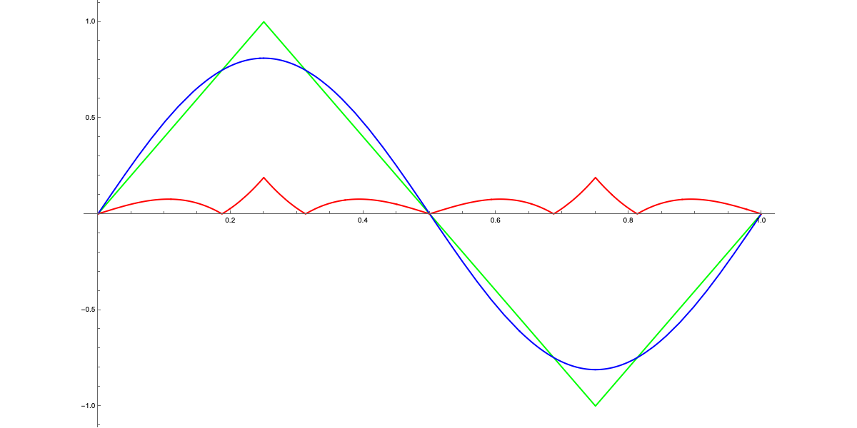
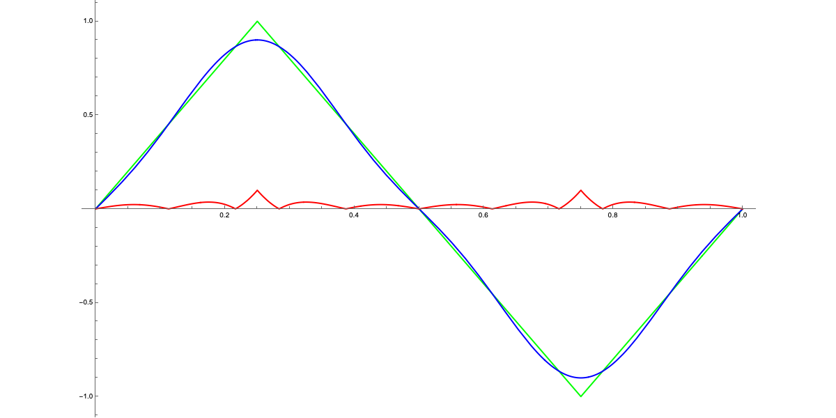
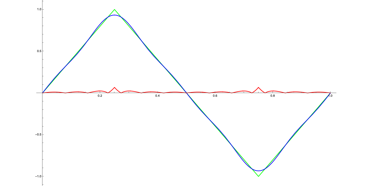
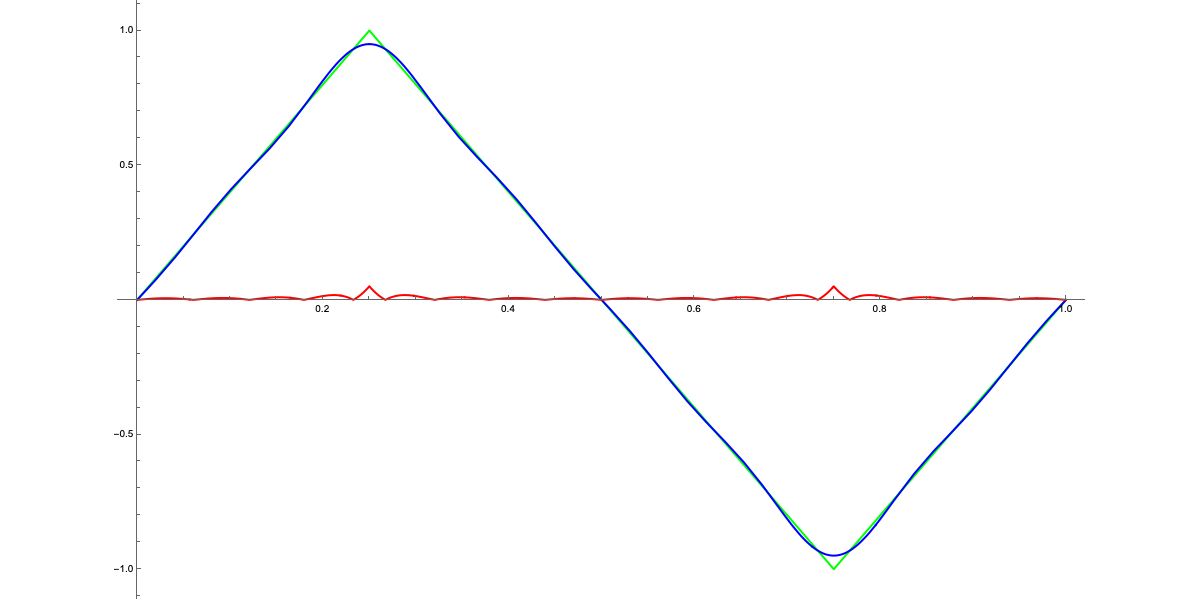
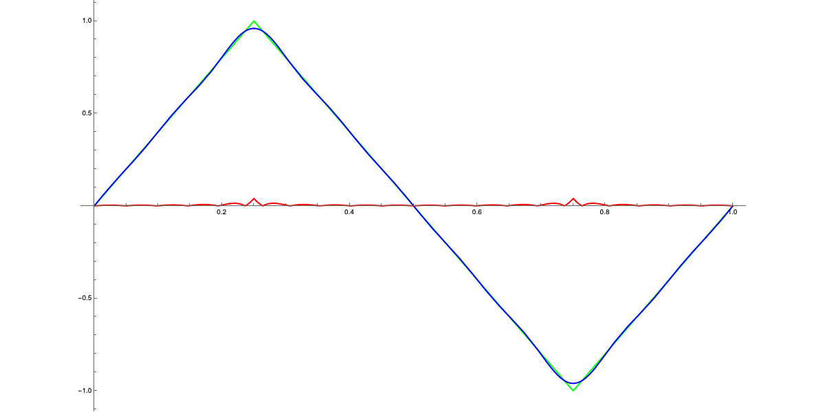
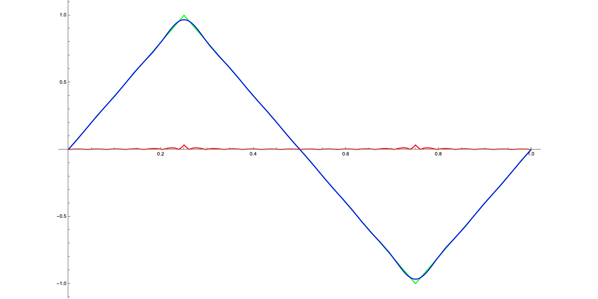
It's possible to observe that for $k>6$, the contribution of the next term changes the resulting frequency only minimally. As good reverse engineers, let’s run an experiment. On Wikipedia's Triangle Wave page, we find the function that defines the triangle wave:
$$ x(t)=x(t)=4\left|t-\left\lfloor \frac{3}{4}+t\right\rfloor +\frac{1}{4}\right|-1$$
and we note that for every positive integer $n$, the partial Fourier series is given by:
$$F_{N}(t)=-\frac{8}{\pi^2} \sum_{k=1}^{N} \frac{(-1)^{k}}{(2k-1)^{2}}\sin\left(2\pi(2k-1)t\right)$$
Now, the Mathematica code that implements all this is:
 x[t_] := 4*Abs[t - Floor[t + 3/4] + 1/4] - 1
 F[t_, N_] := -(8/Pi^2)*
  Sum[((-1)^k/(2 k - 1)^2) Sin[2 Pi (2 k - 1) t], {k, 1, N}]
Let’s observe how the graphs of the Fourier series change as $N$ varies. This is a somewhat informal exercise in the sense that, formally, we should evaluate the mean square error function—but let’s allow ourselves to proceed like this :)
We can notice how the difference between the two curves, shown in red on the graphs, decreases as $N$ increases. As mentioned earlier, for $N>7$, the difference becomes hardly perceptible at a sonic level (in this particular case, I doubt the curve is audible, but let’s let that slide). In any case, this exercise demonstrates that, essentially, a curve (in the mathematical sense, not the "usual" one—it can even be a sequence of line segments) can be very well approximated by a "sum of waves" properly chosen. These observations will be very useful in future articles, but for now:
IF YOU'RE A "Techie": Well, this exercise probably didn’t tell you much that you didn’t already know. You’re already familiar with the power of Fourier analysis and how a complex function can be approximated by a sum of sinusoids. Nevertheless, it remains an important reminder of how central this concept is in so many fields of technology, from telecommunications to audio compression.
IF YOU'RE NOT A "Techie": The key concept is that a sound is essentially a waveform, and that waveform can be approximated as a sum of simpler waves. This might seem like a technical detail, but it’s actually one of the most important ideas in modern mathematics. Think about it: telecommunications, the internet, digital music – all of these rely on this simple idea of breaking down and reconstructing complex signals with simpler waves!
In any case, a quick practical test shows that after $N=5$, the contribution of further terms in the Fourier series is hardly noticeable. So let’s stick with $N=5$ as the maximum value.
Now, back to our friendly musical notes. We’ve seen that a wave at 440 Hz and one at 880 Hz correspond to the same note (A or La), just at two different octaves. In a previous article, I discussed the concept of timbre and how it is made up of harmonics, which are integer multiples of the fundamental frequency. Since we agreed that $N=5$ is a good stopping point, we will primarily consider the frequencies 440, 880, 1320, 1760, and 2200 Hz.
We’ll later explore how these harmonic frequencies are related to the starting note and how they "sound good together," forming what we perceive as consonant chords. For now, let’s ignore 880 Hz and 1760 Hz, as they are simply octaves of our A. This leaves us with the frequencies of 1320 Hz and 2200 Hz, which require closer attention.
Let’s begin with 1320 Hz. We normalize this frequency by bringing it back to the reference interval $[440,880]$:
$$\frac{1320}{880}=1.5=\frac{3}{2}$$
This ratio is of fundamental importance. If we multiply 440 Hz (our A) by 1.5, we get approximately 660 Hz, which is very close to 659.2 Hz, the frequency of the note E (Mi). In musical theory, the interval between A (La) and E (Mi) is known as the perfect fifth.
The fifth interval is crucial in Western music and many other musical traditions. It is one of the most consonant intervals, used to build chords and harmonic melodies. This mathematical ratio, 3:2, forms the basis of scales and chords found in many musical genres. The reason the perfect fifth sounds so harmonious with the fundamental note is that the frequencies are in a simple proportion, which is pleasing to the human ear.
The Pythagoreans discovered that simple numerical ratios produce sounds that the human ear perceives as harmonious. The 3:2 ratio, which defines the perfect fifth interval, was particularly important in their musical theory because it created an extremely consonant sound when two notes were played together. This discovery led to the so-called Pythagorean scale, which is entirely built on perfect fifths and, therefore, on 3:2 ratios.
According to legend, Pythagoras noticed these relationships by observing the sounds produced by hammers of different sizes, discovering that precise mathematical ratios existed between the notes they produced. While this is likely more myth than historical fact, the idea that numerical proportions govern musical harmony became a fundamental principle of Pythagorean philosophy.
The perfect fifth, in particular, was considered so important that it became the foundation of the diatonic scale used in Western music. This 3:2 ratio remains at the core of modern tuning and musical scales, even though the system of equal temperament (which divides the octave into 12 equal parts) became established more recently.
For the Pythagoreans, music was not just an art form but a tangible manifestation of the numerical order that governed the universe. They viewed music as an example of the concept of the "harmony of the spheres," believing that the movements of celestial bodies mirrored similar musical proportions, creating an invisible cosmic symphony.
Thus, the perfect fifth originates from the Pythagoreans and their approach to music as a form of applied mathematics. This legacy is still clearly visible in contemporary music.
However we are terrible and hate Pythagoras :) so let’s divide 2200 by 880, which gives us 2.5, or 5/2. Since 5/2 is greater than 2, we can't use it directly, but we can take the note from the lower octave—just divide by 2! This gives us a new note at 550 Hz, which is close to 554.4 Hz, the frequency of C# (C sharp). This interval is known to musicians as a "major third."
Alright, we now have four notes. Let’s look for the remaining three. Between A and C#, the ratio is 5445. And between C# and E? Well, 3/2÷5/4=3/2×4/5=6/5. Obviously, 6/5<5/4. This leads to the identification of two types of intervals, called MAJOR INTERVALS and MINOR INTERVALS. What we've just defined is the so-called A Major chord (A, C#, and E), which consists of the fundamental, a major third, and a perfect fifth.
The difference between these intervals is crucial for understanding the structure of chords and the quality of musical scales. Major chords, like A Major, are built on major intervals and have a "bright" and open character, whereas minor chords (which involve minor thirds) tend to have a more melancholic or "closed" sound.
At this point, one might ask: I placed a major interval after the A. What if I placed a minor interval before it? Let's divide 440 by 6/5, which gives us 366.67 Hz—this is outside our reference range, but we know that by doubling it, we get something useful: 733.33 Hz, very close to the 740 Hz of F# (F sharp). Since I divided by 6/5, which is equivalent to multiplying by 5/6, and then doubled it, I now have a new factor, which turns out to be 5/3. On the other hand, by taking the perfect fifth (remember, the frequency was 3/2 of the tonic’s frequency, i.e., 440 Hz for A) and multiplying it by 5/4 for the minor interval, we get a multiplier of 15/8, which equals 825 Hz. This is very close to the 830.6 Hz of G# (G sharp).
As I write this, I realize I may have tested your patience, and I hope you recall something from your middle school music lessons! If you’re not familiar with sharps and flats, don’t worry too much: the important thing is to understand that we’re playing with frequencies, raising or lowering them by small amounts.
Now here’s the fun part: all this interval talk doesn’t have "accidentals" (and I’m not talking about sharps and flats) if you do everything in C (Do). It’s the magical key where everything simplifies. Next time, when we delve into the world of accidentals, everything will seem much clearer… I promise! ;)
The final effort remains—let's repeat the game we played earlier. What happens if we precede the newly defined intervals with their duals?
First, let’s add a minor interval to the 15/8 interval we found earlier, meaning we multiply it by 6/5, resulting in 9/4. We divide by 2 again to bring it back to our reference interval, giving us 9/8. Now, 440×9/8=495, which is very close to 493.8 Hz, the frequency of B (Si).
Now, let's precede the minor interval before A with a major one. So, let’s start again: 440÷(6/5)÷(5/4)=440×2/3=293.33 Hz, which, when brought back to our reference interval (by doubling the frequency), gives us 586.66 Hz, close to D (587.3 Hz).
And here are the seven notes! To tease the mathematicians—a group I aspire to join before my demise—I’ll write, "We leave it as an exercise for the reader to verify that repeating the algorithm results only in familiar notes."
We have identified the following notes:
- A (La) – 440 Hz
- C# (Do#) – 554.4 Hz
- E (Mi) – 659.2 Hz
- F# (Fa#) – 733.33 Hz
- G# (Sol#) – 825 Hz
- B (Si) – 495 Hz
- D (Re) – 586.66 Hz
Incidentally, this corresponds to the A Major scale:
The A major scale consists of the following notes:
- A (La) – Tonic
- B (Si) – Major second
- C# (Do#) – Major third
- D (Re) – Perfect fourth
- E (Mi) – Perfect fifth
- F# (Fa#) – Major sixth
- G# (Sol#) – Major seventh
- A (La) – Octave (the tonic repeated one octave higher)
Interval structure of the major scale:
The major scale has a fixed interval structure between each pair of notes:
Whole tone – Whole tone – Semitone – Whole tone – Whole tone – Whole tone – Semitone
Now, let’s try it starting from C (Do):
C, D, E, F, G, A, B, C
What sorcery is this??? Nothing more than what I told you earlier—we just started from C instead of A.
Actually, today we use what is called 12-tone equal temperament, based on the formula:
$$f(n)=440×2^{n/12}$$
where $n$ is the number of semitones away from the central value, the 440 Hz of the note A (which explains why I started from A instead of C).
| Note (Latin) | Alternative Notation | Exponent | Frequency Formula |
|---|---|---|---|
| A (La) | n/a | 0 | |
| A# (La#) | Bb (Si♭) | 1 | |
| B (Si) | C♭ (Do♭) | 2 | |
| C (Do) | B# (Si#) | 3 | |
| C# (Do#) | D♭ (Re♭) | 4 | |
| D (Re) | n/a | 5 | |
| D# (Re#) | E♭ (Mi♭) | 6 | |
| E (Mi) | F♭ (Fa♭) | 7 | |
| F (Fa) | E# (Mi#) | 8 | |
| F# (Fa#) | G♭ (Sol♭) | 9 | |
| G (Sol) | n/a | 10 | |
| G# (Sol#) | A♭ (La♭) | 11 | |
| A (La) | n/a | 12 |
These values are official in the equal temperament system because they ensure that:
- Each semitone is equally spaced from the next, both mathematically and acoustically.
- Each octave exactly doubles the frequency compared to the lower octave.
- Instruments can be tuned to sound good in any key, avoiding excessive dissonances, as happened with other tuning systems.
In the past, systems like Pythagorean tuning or just intonation were used, which were based on simple harmonic ratios. However, these systems presented problems when playing in different keys. Equal temperament solves these issues, although it requires a compromise in the purity of intervals.
Additionally, they provide a rather strict definition of semitones or accidentals.
In conclusion, as we’ve seen, mathematics is closely intertwined with music and acoustics, governing not only the notes we play but also how we perceive sound. Whether it's harmonies, intervals, or frequencies, there’s always a formula explaining what our ears naturally embrace. However, like in all things, there’s always a trade-off: equal temperament made it possible to sound good in any key, but at the cost of pure harmonic ratios.
And it doesn’t end there. The world of sound waves and frequencies opens the door to another mathematical frontier: the difference between discrete and continuous, and the sampling process. We’ll soon dive into the world of Sampling and Aliasing, exploring how signals can be digitized without losing their essence. In detail, the next post will be about sampling and Mr. Knowitall.
Stay tuned! 😄
PS: I’m racking my brain trying to find ways to insert formulas into HTML tables, and to translate physical concepts into something understandable—giving meaning to something that already has meaning, but is truly hidden within the folds of reality. So… maybe you could sign up for the newsletter, right? It’s free, after all!